To introduce the function generator/arbitrary waveform generator and the oscilloscope. You will familiarize yourself with different waveforms and learn how to select a waveform and adjust its frequency and amplitude. You will use the oscilloscope to display the waveforms and to measure their characteristics (amplitude, frequency, phase, rise and fall times, period and offset voltage).

Background:

1.  Function generator 

Up to now we have worked with DC (direct current) voltage and current sources (i.e. power supplies), whose values are constant. In this lab you will become familiar with sources that vary as a function of time (called AC or alternating current sources). There are many different AC waveforms. The one you are most familiar with is the sinusoid as shown in  Figure 1.

Others are the pulse train, triangular and ramp waveforms. The questions we would like to answer in this lab are how to generate these AC voltages and how to measure or display them. We will be using two different instruments: (1) function or waveform generator and (2) oscilloscope. Both are among the most important instruments in electronics. It is essential that you know how to use both instruments well.

In previous labs we have used the digital multimeter (DMM) to measure DC currents and voltages. The DMM in the AC Mode can be used to measure the RMS value of a waveform (root mean square). However, there are many other attributes of an AC signal besides the RMS value that are important such as the exact shape, frequency (or period), offset voltage, phase, etc. as is shown for a sinusoid in Figure 1.

2.  Analog Oscilloscope

One of the most used instruments in the lab is the oscilloscope which allows you to display ("see") the waveform as a function of time in a similar fashion as is done in Figure 1. The oscilloscope consists of a display tube on which one can trace the waveform. An electron beam, which is deflected by electric fields, writes figures on the fluorescent screen. Figure 2 shows the block diagram of the major subsystems of an oscilloscope.

Figure 3 shows the physical details of these subsytems:

The probes are used to apply the signals that we wish to view to the deflection plates which in turn control the horizontal and the vertical positions of the electron beam such that the spot on the screen provides a stationary display of these signals. The function of each of these subsystems will be described in detail below.

There are two types of scopes, the analog and the digital ones. Digital scopes have more features than the analog scopes. Digital scopes can process the signal and measure its amplitude, frequency, period, rise and fall time. Some of them have built-in mathematical functions and can do fast Fourier transforms in addition to capturing the display and sending it out to a printer. The oscilloscopes in the EE Lab are HP 54600 digital oscilloscopes which have most of the above functions built-in. The goal of this lab is to learn how to use the different features of the digital oscilloscope.

2a Scope Probe

A probe is a high quality connector cable that has been carefully designed not to pick up stray signals originating from radio frequency (RF) or power lines. They are used when working with low voltage signals or high frequency signals which are susceptible to noise pick up. Also a probe has a large input resistance which reduces the circuit loading. A probe usually attenuates the signal by a factor of 10. Figure 4 shows a typical probe.

2b. Display Subsystem (CRT)

The electron beam is generated by a cathode which is made out of a material which emits electrons when heated to a high temperature (See Figure 3). The resulting electron beam is focused, accelerated and its intensity is controlled by a grid that surrounds the cathode. The intensity can be adjusted by a knob marked INTENSITY on the front-panel of the oscilloscope. This entire assembly is refereed to as Electron Gun and is enclosed in a glass tube (the cathode-ray tube), under high vacuum. The screen of the CRT is coated with fluorescent material. When the electron beam hits the screen a spot of light is created. This spot is at the center of the display screen unless a voltage is applied to the vertical or horizontal deflection plates.

2c. Vertical Deflection Subsystem

Figure 7 shows the components of the vertical subsystem.

 The signal to be displayed is applied to the input of this subsystem which is called channel 2. Many signals have a dc component. If we wish to display the dc component also, the dc selector switch is chosen. Otherwise we chose the ac setting and the capacitor will block the dc component. The combination of the preamplifier and amplifier is designed to provide a fixed again of usually K=1000. Since we desire to display signals of various strength, by setting the attenuator level, F, at different values, we can achieve an overall amplification of FK for the input signal. Therefore the voltage apllied to the vertical deflection plate, Vvd, is given as,

However, rather than calibrating the input of the scope in terms of the overall amplification, the scopes are calibrated in terms of sensitivity. A knob labeled Vertical sensitivity (Volts/DIV) allows the user to set the value of the input required for a specific vertical deflection, e.g., 1V/div, 1mV/div, etc. If the scope is being used in y-t mode, i.e., a waveform is to be displayed as a function of time, it may be necessary to use part of the input signal to initiate a sweep signal that will be applied to the horizontal deflection plate to move the spot across the screen as time increases (See section 2d ). It usually takes a finite amount of time for this portion of the input signal to make its way through the time-base circuitry, we need to delay the application of the input signal to the vertical plates by the same amount of time. This is achieved by placing a delay line between the amplifier and the vertical plates.

Sometimes we may wish to display two different signals simultaneously. The scopes with dual-trace feature have two preamplifier sections called channel 1 and 2. Each of the signals to be displayed is applied to one the two channels 1 and 2. The output of these channels is periodically, applied two the vertical amplifier using an electronic switch. There are two possible mode for display of these signals. In the alternatemode , in each cycle of the sweep waveform, only one of the two channels is connected to the vertical amplifier. In the chopped mode , at a frequency of about 100kHz, a small portion of one channel followed by a portion of the other channel is repeatedly applied to the amplifier during the same cycle of the sweep. In some scopes on can display the difference of the signals applied to channels A and B.

2d. Horizontal Deflection Subsystem

Figure 8 shows the typical horizontal subsystem. This section has two modes of operation, external and internal trigger modes. In the external trigger mode a signal is applied to the input of the horizontal subsystem (Z) by setting the mode switch to external. After being amplified, it is applied to the Horizontal deflection plates.

 Figure 8. The horizontal deflection subsystem

In the internal trigger mode,a sweep pulse is generated internally and applied to the horizontal plate. Figure 9 shows one cycle of the sweep pulse.

Figure 9. The sweep pulse

 At the start of the pulse, the spot on the screen is at right hand side of the display. If no signal was applied to the vertical deflection plate, during the period t=0 to t=t1 the spot will move horizontally from the left to right at a constant rate. If a signal is also applied to the vertical plates, the spot on the screen will trace a curve corresponding to the signal. During the short time period t=t1 to t=t2 (Fig. 9.), the spot will return to its initial position. During this period the beam is cut off so we cannot see the return portion. Figure 10 shows in detail of the operation during one period of the sweep. The Time/Div switch is used to control the length of the sweep pulse.

 There are two additional steps required. One is to generate the sweep waveform repetitively (triggering) , so that the trace will be drawn over and over again, appearing continuous to the eye. The second is to synchronize the beginning of each sweep pulse with the signal applied to the vertical deflection plate.

We will now see how triggering works ( Figure 11). A periodic waveform such as a sine wave or a triangular wave is apllied to a pulse generator. The pulse generator is set such that every time the triggering signal has reached a specific level, either with positive or with negative slope (one or the other), the pulse generator emits a pulse.

We can set the point at which the pulse generator puts out a pulse by setting a trigger level and choose either a positive or negative slope. These are done by the using the Trigger Level and Trigger Slope switches. In Figure 11, the triggering level is set at the value of the blue horizontal dashed line and the slope is set as negative. Therefore, only the points shown in blue result in the pulse generator emitting a pulse and the green points either do not have the correct level or have positive slope and therefore do not generate a pulse. We also see that not every pulse leads to a sweep waveform. This allows us to choose the sweep length so as to be able to display more than a single period of the input signal.

The second function of the timebase circuitry is to synchronize the beginning of the signal to be displayed on the screen with the sweep pulse. This is necessary to obtain a stable image and is achieved in three different ways.

Internal triggering is when a portion of the signal applied to the vertical deflection plates is used as the triggering signal and fed to the pulse generator. External triggering is when an external signal whose frequency can be set as either an integer multiples or whole fraction of the input signal frequency. Line triggering is when the 60 Hz voltage from power line is used as trigger. There is a default Auto trigger setting that is best for most applications.

Digital Storage O'Scopes (DSOs):

One of the draw-backs of the conventional analog scope is their inability to deal with very low frequency signals. In these cases the spot on the screen would fade before the sweep has had a chance to trace the entire signal and as a result the display would not appear as a solid line. In addition, it is often very useful to be able to store and retain the a signal for a period of time. Digital scopes allow both this goals to be achieved. Furthermore, the stored waveform can be analyzes for many of eats parameters such as rise time, fall time, mean value, rms value, etc. Figure 12 show the major building blocks of a digital storage scope.

 The analog input signal is amplified and sampled and digitized by means of a A/D converter. It is then stored in a memory chip. This information can down loaded to a computer or be transferred to other instruments controlled by GPIB. The stored waveform is then sent to a D/A converter and displayed on the CRT. The content of each location determines the vertical position of each dot on the CRT and the address determines its time-base. The voltage resolution of the scope is determined by the number of bits of the A/D converter and the time resolution is governed by the amount of memory allocated to each waveform stored.

In-lab assignment:

A. Equipments:     

1. Identify the three main blocks of the HP 54600 oscilloscope:

• Vertical deflection system: two input channel coax connectors, vertical scale (Volts/div) and position knobs
• Horizontal deflection system: time base with knobs in Time/div, delay
• The trigger system: trigger source, mode , slope/coupling buttons and trigger level knob
      Also notice the measure and storage panels.

2. Select, display, measure a sinusoidal waveform:

a. Use the HP 33120A function generator to create a sinusoidal waveform with a peak-to-peak amplitude of 1Vpp and frequency of 1 kHz.

b. Connect the OUTPUT of the function generator to the INPUT of the oscilloscope (Channel 1) using a coaxial cable. Push the AUTOSCALE button on the Measure panel. You can switch the input channel 2 off by pressing the button marked 2 on the vertical panel; then push the Off/On key underneath the display window.

c. Change the scale (V/div) of channel 1 (V/div knob, vertical panel) and note the display changes. Try out a few other settings. You can now change the time base as well (Time/div on the horizontal panel). Read the peak to peak value of the sinusoid using the scales of the scope display (shown at the top left corner in V/div). Notice the difference with the setting on the function generator. Explain the difference (hint: output impedance of the function generator is 50 Ohms - see Function/Waveform Generator Tutorial).
NOTE: In case the value of the displayed waveform is off by a factor of 10, check the probe setting. Push the button labeled "1" (channel 1) just above the "Position" knob. This will bring up a menu at the bottom of the screen. At the right hand side you will see Probe 1 10 and 100. Make sure that this is set to 1 (unless you use a probe).

a. Display on channel 1 a sinusoid of a few kilohertz and a few Vpp in magnitude.

b. Select the trigger SOURCE key (on the trigger panel); you will notice a series of choices displayed at the bottom of the screen. Push the key underneath the word Channel 2. This will select channel 2 as the trigger source. Notice and record what happens. Why? Next, select channel 1 as the trigger source.

c. Now change the trigger mode by pressing the MODE key and selecting Auto (with the keys at the bottom of the display). Turn the trigger LEVEL knob to change the trigger level (on the trigger panel) and notice what happens. Can you explain it? What happens when the trigger level exceeds the peak voltage of the sinusoid? Next, select Norm trigger mode (at bottom of the display).

d. Select trigger Slope/Coupling key on the trigger panel. Switch between the positive and negative going slopes. Note the effect on the display.

a. Select a square wave on the function generator with an amplitude of 1Vpp, offset voltage of 0.5V (so that the waveform lies between 0 and 1V), frequency of 1.25 MHz and a 25% duty cycle.

b. Push the VOLTAGE key on the measure panel. Select one of the keys at the bottom of the display to measure the peak-to-peak voltage ( Vpp), average (Vavg) and RMS (Vrms) voltage. Compare and record the Vpp to the RMS values. What is the relationship between both? Now, push the Next Menu button at the bottom of the display. You can now measure the Vmax, Vtop, Vmin and Vbase values. Record these values in your notebook. What is the difference between Vtop and Vmax? Also measure the overshoot of the signal.

c. Push the TIME key on the measure panel in order to measure the frequency, period, rise and fall times. Choose the timebase such that you see one or two periods on the screen.  Select the appropriate keys to measure the frequency (compare with the setting on the function generator), the period and duty cycle. Record these values. Then go to the Next Menu to measure the rise and fall times.

d. Use the cursors to measure time or voltage differences. Push the CURSOR key on the measure panel. Two vertical position-controllable cursors appear and can be used to make time measurements anywhere along the displayed waveform. Use the cursors to measure the pulse width and pulse period. Calculate the duty cycle and compare with the measurement result in part c. Experiment on your own. Similarly, two horizontal cursors are available for precision voltage measurements.

e. Delayed sweep function: in order to zoom in on a specific part of the waveform you can use the delay function. Experiment with this feature. Push the MAIN/DELAYED button on the horizontal panel. Next, select Delayed and notice the display. Change the timebase (Time/div) to further zoom in on the rise time of the waveform. This feature is convenient to look at the detailed structure of a waveform. You can go back to the regular display by pushing the Main display.  

Frequency sweep. Create a sinusoidal waveform of amplitude 1.25Vpp whose frequency sweeps between 50 Hz and 5000 Hz. Consult the user's manual at your station to find out how to do so. Observe the waveform on the oscilloscope. Display the waveform on the oscilloscope.

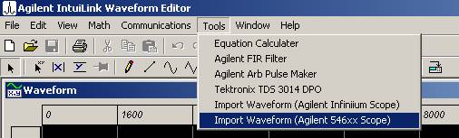
You will use IntuLink Waveform Editor to create your own waveform, store it in the function generator's memory, display it and listen to it. Use the freehand, a drawing pallets or any other tool to create your own waveform. Be creative and remember you will have to listen to it ... After creating the waveform load it into the function generator's memory (using the Send Waveform in IntuiLink Wfm Editor). Display it on the scope and listen to it at the same time. Change the frequency and amplitude and observe the difference.

7. Scope Probe

A scope probe is used to display high frequency signals and to reduce noise and ringing on the signal. In the following experiments you will study the effect of using a probe.

a. Scope Probe Adjustment

Probe pins can be easily damaged or broken. Handle the probe with care.

Connect the probe to one of the input channels of the oscilloscope. You need to inform the scope that you are using a 10:1 probe. This is done by pushing the key labeled 1 or 2 on the vertical panel of the scope and then pressing the key at the bottom right side of the display until the 10 indicator is highlighted

Attach the tip of the scope to the square wave reference signal at the terminal on the front panel (underneath the display indicated by the square wave icon). View the square wave signal on the scope. If the probe is not properly adjusted the square wave won't have square corners. Use your screw driver to make adjustments on the probe so that the square wave has a flat top. Do this carefully and do not turn the screw too much as this can damage the probe. The probe is now ready to be used.

b. Measuring of a square wave

Set the waveform generator to a square wave with a frequency of 2 MHz and 2 Vpp. Display the square wave on the oscilloscope using a coax cable (black cable). Notice that the square wave is not very clean and that it has a considerable amount of ringing.
Next use the probe scope to display the signal. Connect the probe input to the output of the function generator. Be extra careful not to bend the probe pin (it is easily damaged). Also, connect the gound of the function generator to the ground connector of the probe. Adjust the vertical scale of the scope and notice the waveform. It should be much cleaner with less ringing.

c. Effect of poorly adjusted probe

 Lets study the effect of a poorly adjusted probe. Connect the probe input to the output of the function generator (make sure that the ground of the function generator is connected to the probe ground). Select a 2 MHz square wave of 10 Vpp and display it on the scope. Use the cursors on the scope to measure the wavefrom characteristic: peak-to-peak value, Vtop, Vmax. Record the values in your lab notebook. Now mis-adjust the scope probe by turning the screw in the scope compensation box by about a quarter turn. Notice what happens to the square wave output. Do the same measurement as before, record them in your lab notebook. How does it compare with the measurement of a compensated probe? Now readjust the probe carefully, using the reference square wave signal at the scope terminal.
 

Created by Jan Van der Spiegel (jan@ee.upenn.edu), March 12, 1997;
Updated by Jan Van der Spiegel, March 30, 1998.
UNIVERSITY of  PENNSYLVANIA
DEPT of  ELECTRICAL ENGINEERING