 The
alias theorems:
The
alias theorems:
practical undersampling
for expert engineers
Aliasing, long considered an undesirable artifact of an insufficiently high sampling rate, is in fact a useful tool for lab testing and analysis.
Leslie Green, Gould-Nicolet Technologies
Physicist and engineer Harry Nyquist's 1928 paper on telegraph-transmission theory revealed that complete reconstruction of an N-element signal is possible if you know N/2 sinusoidal components (Reference 1). This theory developed into Nyquist's sampling theorem, which states that complete reconstruction of a waveform is possible from samples taken at a rate greater than twice the highest frequency-harmonic component. If you sample the signal more slowly, an alias results, and information is lost.
The alias is unknown to novice engineers, feared by intermediate-level engineers, and used by expert engineers. Certain conditions are necessary to use these advanced measurement techniques, and simple test methods can reveal otherwise immeasurable time-domain characteristics.
Apparatus and background information
For sampled data systems, you need both a sampling system and a signal to sample. DSOs (digital-storage oscilloscopes) have distinct advantages for the description and verification of sampling phenomena because of their crystal-controlled switched-range timebases, displays, and measurement cursors.
A few words of warning for those wishing to test these findings on their own equipment: You must disable any form of peak detection, which your equipment may refer to as envelope detection, maximum-minimum mode, or glitch detection. Next, disable any advanced dot-joining features, such as sine or sinc interpolation; you need linear interpolation for these tests so that you can see the real sample points. Finally, disable any antialias filters that are available to the user. Equipment that does not allow users to disable any internal antialias filters is unsuitable for these tests or measurements.
Analog-sampling oscilloscopes can help demonstrate the idea of correlated undersampling. They are relatively obscure devices for average engineers, partially because they can require significant skill to produce something other than a screen full of disconnected dots. Analog-sampling-oscilloscope technology has existed for many decades and has achieved bandwidths in the gigahertz region. Analog-sampling oscilloscopes are entirely different from DSOs. Analog-sampling oscilloscopes take samples at a rate of perhaps 100,000 samples/sec and yet display waveforms with gigahertz and greater repetition rates. Clearly, analog sampling oscilloscopes take much less than one sample per waveform cycle, yet they manage to reconstruct time-domain signals with a defined accuracy.
How do analog sampling oscilloscopes achieve this accuracy (Figure 1)? The trigger event occurs several dozen nanoseconds ahead of the sample point and initiates a variable monostable that causes successive sample points to occur at an increasing distance from the trigger event. Thus the analog sampling oscilloscope can build up a stable display of a waveform, which is many times faster than the sample rate. For example, a modern, 50-GHz-bandwidth analog sampling oscilloscope can display 10-GHz-repetition-rate signals using a 100,000-sample/sec sampling rate. This ability is an example of correlated undersampling, because a trigger exists, and the sample point moves deterministically through the waveform.
DSOs employ a different technique. For a DSO sampling at 500M samples/sec, the sample points are 2 nsec apart. Thus, timebase speeds in which the screen displays more than 2 nsec use multiple points from one acquisition sweep. A random-sampling system addresses the desire to display the edge of the waveform without using an external delay line to get the advanced trigger. The DSO acquires a waveform at random, measures the time interval between the trigger signal and the internal timebase, and then figures out where to position the acquired point in a reconstruction of the waveform. This well-known technique is called ETS (equivalent time sampling), and you can define it as a form of postcorrelated undersampling in which sample acquisition occurs prior to determination of its time position.
Trigger system
It is important to know what sort of trigger system your acquisition system is using. There are two distinct types. The first, and most common, system is the analog trigger. With this system, an analog signal feeds an analog-trigger comparator, and the level crossing a particular threshold generates a trigger pulse. Many variations on this theme exist, including pulse generation when the signal is outside a range or too small, but all systems based on analog signals are generically grouped as analog triggers.
Digital-trigger systems, in contrast, are systems in which any trigger comparison takes place on the digital data stream that the main channel ADC creates. It is often difficult to notice any functional difference between these analog- and digital-trigger systems for a waveform that is within the range of the display. If you can't find the manual for your particular system, a few simple tests will enable you to tell whether the equipment has an analog trigger or a digital trigger.
Split a signal into two inputs of the equipment using a T-piece or similar splitter. If you can shift the trigger channel trace completely off the display and still get a stable view of the waveform on the other channel, you have an analog-trigger system. Or, if the system has ETS timebase ranges, it has an analog-trigger system. If you set the trigger-level markers to the middle of a known aliased waveform and the trace is steady, you have a digital-trigger system; an analog-trigger system gives an apparently random trigger point on this test.
The distinction between these two types of trigger systems is important when you are dealing with aliases. Arguably, the analog-trigger system is best when you're trying to avoid aliases, and the digital-trigger system is better when you are deliberately trying to create a stable alias.
Uncorrelated undersampling is popularly known as "aliasing"; the older term "beating" is still also used on occasion. An alarming number of engineers consider aliasing bad, dangerous, unacceptable, and not at all useful. For example, for some equipment, the manufacturer of the sampling system goes to the trouble of limiting the system bandwidth so that aliasing does not bother the users. It is a matter of popular experience that an alias of a sine wave looks pretty much like the original sine wave. What is perhaps less well known is that the alias of a square wave is a square wavebut not just any square wave. The alias is a time-scaled replica of the original, if the alias conditions are correct. This point is very important.
The alias is more easily recognizable on a modern DSO than on one designed 15 or 20 years ago. The tendency now is to have an accurate vertical-trigger-level marker displayed on the screen. Suppose the trigger-level marker is centered on the trace, the trigger coupling is set to dc, and the trigger light is on, but the waveform is unsteady. This situation is a clue that aliasing is occurring. Of course you still have to check that you are triggering on that channel! Note that this clue applies only to analog-trigger systems. If the trigger is developed from a digital comparison against the acquired digital data, then the alias will appear in a stable position on the screen.
In ordinary use, you strictly avoid the alias, and if you find one, you change the conditions to make it go away. You might achieve this objective by increasing the sample rate, selecting some sort of peak detection mode, or filtering the incoming signal. You can also accomplish useful measurements by deliberately aliasing the signal. A few specific uses of aliasing follow. After seeing these applications, you may be more interested in the generalized theory behind the measurements (see sidebars "Definitions" and "Theorems").
Suppose a particular digital-acquisition system has a sampling rate of 10M samples/sec and a bandwidth of 5 MHz. You've measured the bandwidth by a sinusoidal envelope-amplitude method, the standard 3-dB-down bandwidth point. You want to know what the pulse response is like, as this may be adversely affecting the measurements. You expect a 5-MHz bandwidth system to have a rise time of around 70 nsec, as the approximation formula suggests:
![]()
The acquisition points are 100 nsec apart, so there is no chance of evaluating the pulse response of the system. Or is there? If you put a square wave with a repetition rate close to 10 MHz into the system, the resulting alias does not give a good representation of the pulse response. The square wave is just too fast for the bandwidth. The edge does not have a chance to settle out before the next transition. A 1-MHz square wave is more appropriate in this case. The expected rise time of 70 nsec is then a smaller part of the cycle, and you can more clearly see the edges of the square-wave response. However, a 10M-sample/sec sampling rate will not alias a 1-MHz square wave.
Your options are to either turn down the sampling rate on the system, if possible, or to discard nine out of every 10 of the acquired points. This decimation process gives the desired sample rate of 1M samples/sec. Notice that you can do this decimation external to the sampling system, by transferring 10 times as much data as required, then selecting one of every 10 points by using, for example, a Visual Basic program. You need to apply a square wave that has a repetition frequency of slightly more than 1 MHz. If the square-wave frequency were exactly the same as the sampling frequency, you would get, in principle, a straight line. If the square-wave frequency is slightly lower than the sample rate, the alias is a time-reversed and -scaled version of the system pulse response. However, if the square-wave frequency is slightly higher than the sampling rate, you get the desired result.
Using a digital timebase on the sampling system and a synthesized signal generator set to 1.002 MHz, the nominal expected alias is about 2 kHz. You can achieve additional accuracy by measuring the actual alias frequency. A 2-kHz signal has a repetition period of 500 µsec, which is 500 points at a 1M-sample/sec acquisition rate. You measure the displayed frequency of the waveform as, for example, 2.05 kHz, but you know that the actual frequency is 1.002 MHz. Thus, you need to rescale time by the factor
![]()
Multiply the rise time of the aliased square wave by this scaling factor, and you have the rise time of the actual system. Suppose the rise time of the alias measures 35 µsec. You then calculate the rise time of the system using the equation
![]()
The way to solve these types of problems is to initially use a slower sample rate and a lower alias frequency. Then, you can increase the sample rate to 1M sample/sec so that the aliased edge has more points on it. This increase enhances the resolution of the measurement. In any case, the overshoot and shape of the pulse are always correct. Note that if you reduce the alias frequency, less than one complete alias cycle may appear on the 1M-sample/sec range. If the equipment has an analog-trigger system, then you'll probably need more than one acquisition sweep to capture the rising edge. This task is easy when you do it manually. Just keep doing "single-shot" acquisitions until you get one with the rising slope roughly where you want it.
For this sort of test, a digital-comparator-trigger system might actually be preferable, provided it can trigger on the displayed data. Note that if the system acquires at 10M samples/sec, the display may give decimated data at a 1M-sample/sec rate, but the trigger comparison may still be done at 10M samples/sec. Unfortunately, manufacturers' data sheets probably don't provide this level of detail.
Sample-to-sample stability
A crystal ordinarily controls the timebase of a digital-acquisition system to a high degree of accuracy. Although ±100-ppm absolute accuracy was the norm a few years ago, recent advances in crystal technology mean that timebase accuracies of ±25 ppm, ±10 ppm, and better are becoming more common. Novice engineers might therefore think that the time separation between two adjacent sample points is accurate to the published timebase specification. Consider this from a more practical point of view.
On an acquisition system with a sample rate of 500M samples/sec, the interval between dots is 2 nsec. Accuracy of ±25 ppm on this interval gives rise to an uncertainty of ±0.05 psec. This expectation is unrealistic for sample-to-sample jitter in any normal acquisition system. Realize that the timebase specification measures over some longer time intervalperhaps 10 to 100 msec long. Thus, the quoted accuracy is of an average interval and does not represent the sample-to-sample jitter due to phase noise in the master timebase oscillator and jitter in the logic gates.
Because sample-to-sample separation is not a specified, guaranteed, or even measured quantity for most acquisition systems, anyone making detailed time measurements may need to measure his or her equipment to establish the actual jitter. High-end DSOs may have characterized jitter performance, but they are out of the budget range of many users. One method of quantitative evaluation uses an alias.
In this approach, you first need a stable oscillator. The resulting measurement is going to include any jitter due to the phase noise in the oscillator. Thus it is essential that you use the best available generator. The next requirement is to minimize amplitude noise by using an insensitive range on the acquisition system and, correspondingly, a large amplitude from the oscillator. If there is any possibility of spurious components from the oscillator, you can improve noise by using a narrowband-tuned filter. It is simple enough to make up a passive LCR filter with 20-dB extra insertion loss when the frequency is an octave (´2) away from the peak response. This technique improves any spurious noise sources on an already good oscillator.
As before, you are feeding a 1.002-MHz signal into a 1M-sample/sec acquisition system. The only difference this time is that you use a sinusoidal signal. A sinusoidal signal makes it easier to produce a clean, noise-free waveform. With a 2-kHz alias frequency, you should not see any noise or distortion on the sinusoidal signal. As the alias frequency gets lower, however, the effects become much more noticeable. The sinusoid can become highly distorted when you reduce the alias frequency below 100 Hz. In fact, you may then be able to see the effect of analog-trigger breakthrough into the acquisition timebase clock. If your equipment has an analog-trigger system, it is therefore better on these tests to let the acquisition system "free run," rather than to use the signal as a trigger source.
Remember that the alias-to-actual-frequency ratio must scale down in time any perturbation on the sinusoidal signal. If you fill the display with the 1-kHz alias of a 1.001-MHz signal by using a 100-µsec/division timebase, then 0.1 division of jitter corresponds to a real-time jitter of
![]()
That is a huge amount! With a good analog-signal generator and a steady hand, you should be able to take the alias frequency down to 100 Hz or less. Notice that if the 100-Hz alias is displayed across the whole screen by using an acquisition speed of 1 msec/division, 0.1 division of horizontal jitter corresponds to a real-time jitter of
![]()
Notice that the jitter as a ratio of the cycle time of the alias corresponds to the same amount of real-time jitter. You might, therefore, think of the jitter as being constant as you reduce the alias frequency in proportion to the timebase. This constancy does not happen in practice, however. As you reduce the timebase and alias, the jitter increases. At some point, the alias breaks up completely and is not even close to being sinusoidal or even periodic. The point at which alias breakup occurs is a powerful test of the stability of the internal master oscillator and the external oscillator. In fact, you can use alias breakup as a means of comparing different acquisition systems and oscillators.
So far, you have checked the timebase-sampling interval to only 10-nsec resolution. This resolution measurement is poor for a timebase that claims better-than-100-ppm accuracy. You need to put in the low-frequency alias but view it on the faster timebase. The trouble is that the signal will then appear as a straight line. You have to look for vertical deviation from this line, rather than for horizontal jitter. You previously established the vertical noise level of the equipment. Because you are on one of the least sensitive ranges and on a fast timebase, you should expect the noise to be around 1 LSB on an 8-bit system.
Because the signal comprises six divisions point to point, the alias also comprises six divisions peak to peak. You either set the digital trigger to midscreen or, on an analog-triggered system, keep doing single-shot acquisitions until you get one near the middle of the screen. Suppose you see 0.1-division point-to-point noise on this straight line. This vertical deviation corresponds to a phase difference of
![]()
radians and, consequently, a time deviation of
![]()
This deviation then
rescales by the alias-to-actual frequency ratio, so that the alias frequency
drops out of the equation. The timebase jitter is therefore
![]()
The best resolution available for the sample interval measurement in this situation is about 5 nsec, unless you resort to curve-fitting techniques to more accurately estimate the jitter.
Although the resolution
of this sort of test is relatively low, it will still show the weaknesses
in multiphase-acquisition systems, such as CCD-based equipment and systems
that interleave ADCs to get faster sample rates. Resolution of 5 nsec is
not the best this system offers. You could take the amplitude jitter down
to the least-significant-bit level and extract a bit more resolution on
the measurement. However, amplitude and time jitter become indistinguishable
at this level. If the system had a 1G-sample/sec sample rate, then you
should expect to be able to resolve down below the 5-psec level by simple
scaling of the previous results. However, when these numbers run down into
the picosecond region with five-digit resolution, you should be highly
suspicious of the subfemtosecond results that some custom jitter-measurement
software displays!
| Theorems
Philosophers and physicists have observed the general concept of alias phenomena over the ages. Similarly, cinema audiences and TV viewers all have seen the wheels on stagecoaches apparently rotating backwards and propellers on airplanes apparently slowing down, then going backwards. The main text of this article collates these aliasing results into a simple and quantitative form, with specific application to the acquisition of data. The following theorems provide a generalized background for the examples. Frequency-domain alias theorem: For a modulated signal (frequency domain), ideal undersampling loses the carrier-frequency information but does not lose any of the modulation information, provided that the modulation does not extend out from the carrier by more than half the sample frequency. Alias theorem A: If the signal frequency is within 5% of the basic sample rate, there will be at least 20 samples per cycle on the alias. If the signal is within 1%, there will be at least 100 samples per cycle, and so on. In general, a signal within X% of the basic sample rate gives at least 100/X samples per cycle on the alias. Alias theorem B: Decimation by the integer amount D requires that the signal be closer to an integer multiple of the decimated sample rate to get the same number of samples per cycle on the alias. Specifically, being within X% of the nearest integer multiple of the decimated rate gives at least
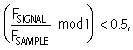
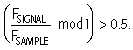
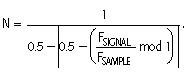
samples per cycle. Alias theorem B is, therefore, a generalization of Alias theorem A. Alias theorem 1: For an ideal repetitive time-domain alias, time-related features on the alias, such as rise time, scale by the ratio of the repetition frequency of the alias to the repetition frequency of the original waveform. Amplitude-related measures, such as overshoot and peak-to-peak aberration, are unaffected by ideal undersampling. Alias theorem 2: You can express the number of samples on each cycle of the alias mathematically as
Alias theorem 3: For a repetitive time-domain signal, ideal positive undersampling loses the repetition-frequency information but does not materially change the shape of the signal, provided that there are at least 10 points on the aliased rise time and that waveform artifacts are not smaller than 1/5 the rise time. Ideal negative undersampling gives a time-reversed but otherwise correct alias (Figure A). By using these alias theorems, you can make some previously impossible measurements with defined accuracy. Also, you can quantitatively evaluate the sample-to-sample jitter of acquisition systems. Rather than being a nuisance, the alias can be a useful tool for sampling systems. |
Author Information
Leslie Green has a bachelor's degree in electrical and electronic engineering from Imperial College (London). He has 20 years of experience working with test-and-measurement equipment, the last 15 years of which he spent designing DSOs for Gould-Nicolet Technologies in the United Kingdom.
Nyquist, Harold, "Certain topics in telegraph transmission theory," Transactions of the AIEE #47 , February 1928, pg 617 to 644.
This
article ran on page 97 of the June 21, 2001 issue of EDN.
Copyright
© 2001 Cahners Business Information, A Division of Reed Elsevier,
Inc.